[Script] Change/reset the foreground color of a block diagram/specific blocks in a block diagram

 There are specific situations where you may want to change the foreground (or even background) of blocks within a Simulink model. In some cases, you might want to revert to a stock color scheme if you've been too... creative with the colors of your diagram (or someone else who had previously worked on the same model has opted for a very colorful model). In other cases, someone might have wanted to highlight changes in a model, but this is no longer relevant since you will now implement your own. Therefore, you will have to revert to a black foreground for all blocks.

Doing this manually would be a tedious job, whereas with a script, it would be almost instantaneous. 

Let's consider the following model, where I've set the foreground color of two blocks to green.

Here's a script to revert all block foreground colors to black.

blocks = find_system('testforeground'); %replace testforeground with your model name if length(blocks)>1 %check that the model is not empty for i = 2 : length(blocks) % the first element is the model itself if string(get_param(string(blocks{i}),'ForegroundColor')) ~= 'black' %replace with == 'color_of_choice' if you only wish to revert specific colors set_param(string(blocks{i}),'ForegroundColor','black') %you may also act upon the background color by using BackgroundColor as the second parameter of get_param and set_param end end end

This is the end result.

Now, let's consider that you wanted to change the foreground color of all blocks of a specific type (let's say, our constant blocks). Here's a variation of the above script that will help you do that.

blocks = find_system('testforeground'); %replace testforeground with your model name if length(blocks)>1 %check that the model is not empty for i = 2 : length(blocks) % the first element is the model itself if string(get_param(string(blocks{i}),'BlockType')) == 'Constant' %replace Constant with block type of your choice set_param(string(blocks{i}),'ForegroundColor','blue') %you may also act upon the background color by using BackgroundColor as the second parameter of get_param and set_param end end end

And here's newly highlighted model.

We can further enhance the functionality, the possibilities are endless. For example, we could create a comparison script between two models, highlighting the added or removed blocks. But that one is for another day.

[Tutorial] Enabled Subsystems and Merge Blocks

 This post is going to be a bit different, as it will not necessarily be focused on a particular application (it will have some context to it, though). I am going to focus on enabled subsystems and how to integrate them with merge blocks in order to compute variables.

First of all, let's start by seeing what a subsystem is: a subsystem is a set of blocks that have been grouped together in order to simplify the representation of a diagram. We will only consider virtual subsystems right now. A subsystem creates a graphical hierarchy and all blocks within are visible and accessible by double clicking on it and accessing the corresponding level of the created visual hierarchy.

We can create an empty subsystem from the Simulink Library and populate it with blocks or we can drag our cursor over multiple blocks, right click and create a subsystem from our selection. If there are unconnected lines or unconnected I/Os of the blocks involved in the subsystem creation, inputs and outputs will automatically be created within the subsystem and connected to these lines/ports.

In the example below, the resulting subsystem (right) will have 3 inputs and one output that will be created automatically.

If no specific scheduling is specified at the subsystem level or a parent level, the calculations within the subsystem will execute every simulation step. While it's ok that we don't have to worry about our subsystem not being taken into account when computing, this behavior is not always ideal.

What if we wanted to compute a variable in two different fashions, depending on a certain situation? One might say that you could use a switch, but it's not always indicated.

What if we had two strategies in mind on how to compute a variable within a vehicle's ECU, but one strategy requires a certain type of sensor (like a camera, for example), that is only available on higher specs of the car? We could construct two different models that would translate into different software components, each to be integrated in the ECU of its respective vehicle configuration, but this would take more time and effort. We would have to maintain and update two models instead of only one, we would have to make sure that the outputs correctly communicate with other SW components in both cases, and in case of a difference in variables names, we might have to include macros in order to correct any deviations in names and such.

In such cases, we usually use a calibration that enables one of two strategies, depending on its value. 

Each strategy could be computed within an Enabled Subsystem. Such a subsystem only computes its outputs when the enabling condition is true.

In order to create an Enabled Subsystem, we could either create it from scratch using the Library Browser, or we could convert a conventional subsystem into an enabled one using an Enable block.

In the example above, I've first created a subsystem that computes the average of two inputs. Afterwards, I've added an Enable block in order to condition its execution. Now, the subsystem will have an additional port on its upper side that needs to be connected, in order for its contents to be executed.

Let's see an example model, in order to better understand how it works.

In the example above, the value of the "Complex_strategy" calibration is used to determine whether Out1 will be the arithmetic average of In1 and In2 or a weighted average (set to 0.4 for In1 and 0.6 for In2). When it is set to 0, we will use the Simplified_comp subsystem. Else, we will use the complex computation in the above subsystem.

Note that both outputs are fed to a Merge block. This block will propagate the output of whichever subsystem is enabled, towards the Scope (it can be any other type of block). Thus, we avoid creating two separate variables, since we only have one output of interest, but computed in two different ways.

Merge blocks are not limited to only two inputs, the user may use as many as he wishes. What is extremely important is to ensure that only one input is propagated towards the merge, at any given time. In our case, we need to ensure that the conditions enabling the two subsystems may never coincide, under any given circumstances.

Let's see an example of how improper conditions may lead to simulation errors. In the example below, step is set to pass from 0 to 5 at 3s. Since the two conditions are not mutually exclusive, they are both met, and both outputs of the two subsystems are fed to the merge block at the same time. This will result in a simulation error, since the model cannot chose between the two.

So, to summarize:

  - there are certain situations where it is preferable to work with Enabled Subsystems (choosing between strategies or applying different operations to the same variable, depending on an external condition);

    - an Enabled Subsystem will only execute its contents while the enabling conditions is true;

    - we can merge the outputs of Enabled Subsystems using a Merge block (whichever strategy is used will be propagated towards the output of the Merge);

    - we must be very careful to ensure that the conditions that compute the inputs of the same Merge block do NOT take place at the same time, under any circumstances.

That should be it for now. Next time, we will take a look at a different approach to compute the contents of Subsystems only under given circumstances, by using function calls.

[Example] Creating a counter hold and reset functionality (State chart approach)

In my previous post, I've implemented a counter with hold and reset features. Although the block diagram isn't complicated, the implementation can be greatly simplified. Given that these are temporal functionalities, a state chart approach is much more suitable for the implementation

1) Objective:

Create a counter with an embedded hold functionality, as well as a reset. The reset takes priority over the hold (even if the hold is kept at a True state, the counter will be reset and start counting if the reset signal is True).

2) Model configuration: 

Solver -> discrete, fixed simulation step. Step-size -> 0.01s. We will use MATLAB as the action language of our chart.

3) Principle of operation

We can distinguish 3 operations that our counter does, therefore there will be 3 associated states:

a) Incrementation -> this means that we will just add the value of a simulation step every time the computation reiterates.

b) Hold -> during this state, the counter will not increment. The beauty of state charts is that we can just implement an empty state, it is not mandatory to propagate a value through the computation chain at every step (something like adding 0).

c) Reset -> we just need to set the counter to 0. However, this is where it gets a bit tricky, as we might offset our counter by 1dt if we don't set the instructions right.

4) Solution

I would like to start with some notes: for this example, the input hold and reset signals are already processed outside the chart in order to get their rising edges. These impulses will trigger the transition from one state to another. We could just implement the rising edge detection inside the chart, in a parallel state. However, I've already covered how to get the rising edge here.

Let's look at the first attempt at the implementation. Note its simplicity, when compared to the block diagram approach.

The default state will be Calc, which will increase our counter. There are two possible transitions from this state: towards hold or reset. Note how reset has 1 on the transition, meaning that the condition will be evaluated before the hold condition. This will prevent losing 1dt by transitioning to hold in case both signals become active at the same time. Also note that the Reset state could have been avoided altogether, but I kept it for legibility.

This implementation has one issue. If we get a reset at 2s, we use 1dt to enter the Reset state. The counter itself is set to 0 one dt later, meaning that our counter becomes 0 at 2.01s. This is not ideal.

Let's try another approach, by moving the {counter = 0;} instruction inside the Reset state.

This creates a new issue. Right now, if we get a reset request at 2s, the counter will indeed be reset precisely at that timestamp. However, we will lose a dt to transition towards the Calc state, with no action taken. This means that, instead of incrementing at 2.01s, our counter will increment at 2.02s.

There is one fix that we can implement.

By adding an additional incrementation instruction on the transition exiting from the Reset state, we will compensate that 1dt delay until we enter the Calc state. Therefore, our counter will work accordingly.

As a conclusion, I would say that even though there are some factors that we must take into account in order to properly tune our functionality when implementing it in Stateflow, this is still a much better optimized solution than working with block diagrams for this particular feature.

[Example] Creating a counter hold and reset functionality (Block diagram approach)

In one of my previous posts, I've written about how to implement a counter in Simulink. While this is a neat features, a counter is rarely a standalone feature.

Maybe we need to count the number of km a vehicle has traveled, or just the time the vehicle was in motion. While the vehicle is stationary, we should stop the count. Maybe if we engage the reverse gear, a new count must be triggered. Since we engage reverse while stationary, chances are that the counter was already held before, so we need to reset it while in a held state.

In this post, I am going these features in a Simulink block diagram. 

1) Objective:

Create a counter with an embedded hold functionality, as well as a reset. The reset takes priority over the hold (even if the hold is kept at a True state, the counter will be reset and start counting if the reset signal is True).

2) Model configuration: 

Solver -> discrete, fixed simulation step. Step-size -> 0.01s. We will use MATLAB as the action language of our chart.

3) Principle of operation

Basically, while a signal is true, the counter will no longer increase. I am also going to implement a reset, that will restart the count based on the rising edge of a signal. Furthermore, in order to increase the complexity, the reset will also override an existing hold (even if the hold is set to True, the reset is going to ignore it and just start the counter all over again).

4) Solution

Let's start by implementing the hold functionality. This one's very easy, we just need a switch that lets us chose between adding the simulation step or 0, while our control signal is true.

The reset works in a similar fashion. We just need to add a rising edge detection to our control signal and implement a second switch instead of the unit delay, so that both the increment and the current value get set to 0 when our reset signal is sent.

The question is: how to implement both? We can see that the diagrams are relatively similar. We could implement a logical OR between the reset and hold signal acting on the upper switch, right? Well, not really. If both the hold and reset would be active, the reset would set our counter to 0, but it wouldn't start rising until the hold signal would fall. We need a different approach.

The hold has two states. If it rises, we are sure it is set to True, whereas if it falls, we are sure it is set to False. No intermediate states exist, so we don't really need the signal itself to control our switch. Therefore, we are going to SET the hold when on its rising edge and RESET the hold on its falling edge or on a rising edge of the reset signal. We will do this using a flip-flop. All this will act on the upper switch. But this upper switch also needs to select 0 when we reset our signal, so the output of the flip-flop will be passed through a logical OR block, along with the reset. It might sound a bit complicated, but it really isn't, once you see the figure below.

In this example, I've tested a standalone reset, a reset that overrides a hold and a standalone hold, in order to ensure that all the functionalities have been validated. 

- The first reset takes place at 2s. 

- At 4, the counter is frozen due to the hold signal. Even though the hold is kept up to 8s, it is not fully taken into consideration as a new reset signal is sent at 7s. 

- A final hold command is requested between 15 and 16s.

NOTE: to simplify the diagram, I've used some subsystems for the rising edge and falling edge functionalities. The content of the subsystems is exactly what's been presented in the previous tutorials on these features.

[Example] Creating a rising edge, falling edge and either change detector (State chart approach - previous value generation inside chart)

    Now that we've discussed a bit about change detections here using a block diagram approach, I would like to show you have this can be achieved using Stateflow. The principle remains the same, but what I'm actually interested in showing you is how to obtain the previous value of a given variable in a chart, without using any unit delay, memory hold or latch (in order to compare it with our current value). Here we go.

1) Objective:

Create a rising edge, falling edge or change detector.

2) Model configuration: 

Solver -> discrete, fixed simulation step. Step-size -> 0.01s. We will use MATLAB as the action language of our chart.

3) Principle of operation

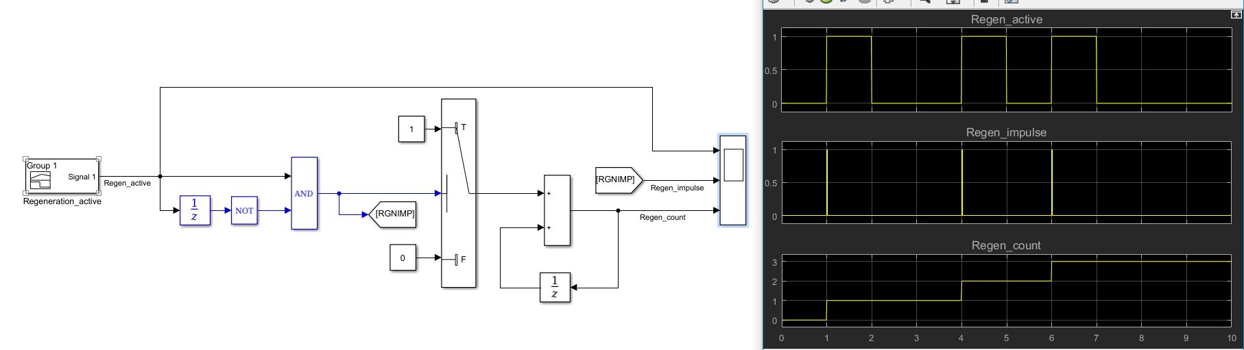
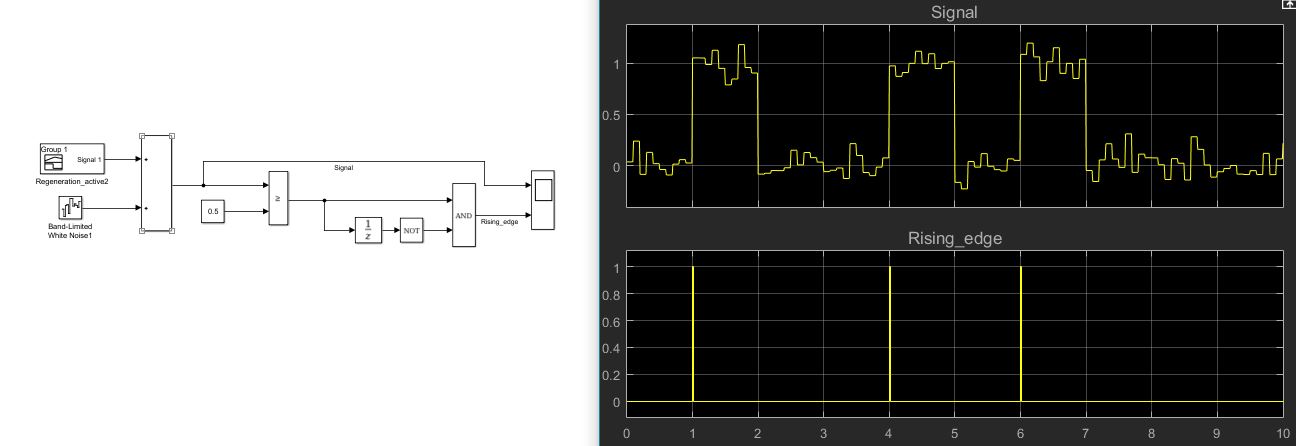
Rising edge -> (x(t-1) == 0) && (x(t) > 0)

Falling edge -> (x(t-1) > 0) && (x(t) == 0)

Detect change -> (x(t-1) ~= (x(t)) (for floating point, abs(x(t)-x(t-1))>tolerance)

Most importantly, we need to learn how to get x(t-1) directly within our chart. It's very simple actually: we will create a local variable. The last instruction performed in the chart at every iteration will be assigning the value of our input to this local. Thus, at the next iteration, our local will hold the previous value of our input.

4) Solutions

Let's suppose our input is an 8 bit unsigned integer. Thus, we will no longer take into account any rounding errors and so on (discussed in the previous example).

a) Create a chart. Using the model explorer, create a variable called SF_input (scope -> input, type -> uint8).

b) Create another variable called SF_input_old (scope -> local, type -> uint8).

c) Create a variable called Sgn_rising (scope -> output, type -> boolean).

By now, you should have something like this:

d) Create a state, name it. Initialize SF_input_old. Without it, we will have a simulation error, as our chart will try to access its value without it being assigned at t=0s. Furthermore, I do not suggest initializing it to 0 (if our SF_input has a constant non-null value, we will detect a rise after 1 simulation step, even though our input hasn't changed). Use SF_input as the initialization value.

e) Start coding the logic. We will use a few junctions. Our condition will be [(SF_input_old == 0) && (SF_input_old > 0)]. Be sure to place this condition on the transition marked with 1, or else the condition will never be evaluated. If the condition is met, we will set Sgn_rising to true, else Sgn_rising will be set to false. After both assignments, remember the most important instruction: {SF_input_old = SF_input;}. This will ensure that our previous value gets updated every simulation step. Here's how your chart should look like.

In case you wonder why I added the second junction instead of placing the instruction under the condition, there are two reasons: first is good practice (conditions should be placed horizontally, whereas assignments should be placed vertically). The second one would be to improve legibility. It's not mandatory to use my approach, though.

Here's the result of the simulation (note that I've added a Data Type Conversion to the step input, as it is a double by default):

Here's the logic for the falling edge (using a new output called Sgn_falling):

And the change detector (using Sgn_change):

That should be it. The main aspect I wanted to focus on was how to create a local that can store the previous value of a variable inside a chart. It's a very useful functionality in a variety of situations (such as the ones above).

[Example] Creating a sliding (animated) tangent plot for a given function (MATLAB)

Basically, this is what we're going to achieve today: 

Why am I interested in this particular example?

It's actually quite simple. This example relates to the notions of slopes and derivatives.

Quite often, in automotive, in case of a failure, we need to ramp-down certain signals (for example, the assistance torque on the steering wheel). We may have requirements stating that the ramp-down must take place with a gradient of x/s or that the signal must reach 0 in y seconds. If we do not have a proper theoretical background, we will not be able to satisfy these requirements.

First of all, what is a derivative (or, better said, what information does it provide us)? Well, simply put, a derivative is a measure of the rate of change of a signal/function, depending on a parameter called the independent variable (for example, speed is a variation of position depending on time). 

The first derivative of a function (no matter the order of that function), will provide us the slope of that function, or the steepness of its graph. By looking at the animation above, we can see that the slope (the magenta tangent) starts quite steep, gradually becomes more gentle, and is quasi-horizontal between -1 and 1, where the function itself is quasi-constant. It then becomes steeper again, when the function starts rising once more. The slope of the tangent line is the same as the derivative of the function at the respective plot point.

What's the mathematical definition of a derivative?

f'(x) = lim h--> 0  (f(x+h)-f(x)) / ((x+h)-x)

What does this formula tell us? 

Well, my interpretation is that if we consider two points that are very close to each other (their difference, h, is infinitesimal), near the graph of the function, we can create a line based on these two points. This will provide us a local tangent to the graph, thus creating the slope of the function for our given point, x. We can also see that this slope is equivalent to delta(y)/delta(x).

So, in order to integrate our knowledge in MATLAB and plot the above figure, we need to:

a) Compute the derivative of our function, in order to get the generic expression of the slope of its tangent line

b) Consider the slope of our tangent line -> slope = (ytg-ytg0)/(xtg-xtg0), where xtg0 will be every point of our x range, and ytg0 the value of our function for that particular xtg0.

c) Write the expression of our tangent as ytg=slope*(xtg-xtg0) + ytg0;

Now we just have to sweep xtg0 through our entire x range in order to recompute the tangent, plot (xtg,ytg), delete it, repeat.

I took some inspiration from this post that shows how to plot a static tangent for a given point, but I've added the extra elements in order to animate the figure. The full code is below (except for the conversion to gif, that one's for another day).

x = linspace(-5,5,100); y = x.^3+1; %Creating a figure object h = figure('Name','Sliding Derivative'); plot(x,y,'b-'); %I am setting the x and y limits of the plot for a better visual effect, %else MATLAB will adapt the limits for each plotted tangent xlim([-5 5]) ylim([-200 200]) %I always use grids, it's a personal preference, but you can disable it if %you prefer grid on for i=-5:(x(2)-x(1)):5 %We need swipe all the x coordinates in order to plot the sliding tangent xtg = i; %The slope will be required in order to compute y, since y-y0 = slope*(x-x0) slope = 3 * xtg^2; %We need to compute the y coordinate of the tangent for corresponding to our current x coordinate ytg = xtg .^ 3 + 1; % Y value of curve at x = xtg. hold on; %It's time to define our tangent line. It will be updated each iteration, %as our xtg and ytg points change ytgln = slope * (x - xtg) + ytg; %I am assigning the plot to an object, in order to be able to delete it %before plotting the next tangent crtplot = plot(x, ytgln, 'm-'); %Once again, I am setting the x and y limits of the plot for a better visual effect, %else MATLAB will adapt the limits for each plotted tangent xlim([-5 5]) ylim([-200 200]) %The pause will define the speed of our animation pause(0.1) %The delete function will delete our currently plotted tangent, %else they will overlap delete(crtplot); end %Closing the figure after executing the for loop close(h)

[Example] Creating a rising edge, falling edge and either change detector (Block diagram approach)

Quite often, we need to trigger a specific action when a change in an input's behavior is detected. Maybe we would like count how many times a certain action takes place (for example, the number of particulate filter regeneration attempts during the same driving cycle). Adding 1 while the regeneration process is active would only increase the counter during the entire process, which would result in a bad count. Consider the example below.

Our counter should have reached 3 when the 3rd regen started, but we can see that we are continuously increasing it throughout the regeneration process. To correct this unwanted behavior, our switch should only receive a 1dt (1 simulation step) impulse when the regeneration process starts, in order to count properly. Let's get started.

1) Objective:

Create a rising edge, falling edge or change detector.

2) Model configuration: 

Solver -> discrete, fixed simulation step. Step-size -> 0.01s.

3) Principle of operation

Let's consider the following sequence: 0,0,0,0,0,x,x,x,x,x,x, where x is a positive number (let's consider it an integer). We want to distinguish the moment when the transition from 0 to x takes place. Therefore, we will model a condition indicating that x(t) is non null and x(t-1) is null. This will be our rising edge detector.

For our falling edge, consider x,x,x,x,x,x,0,0,0,0. We need to detect the moment when x(t) is null and x(t-1) is non null.

The either edge detector will be a mix between the two (rising-edge OR falling-edge). However, we will just simplify it as x(t)~=x(t-1).

4) Solutions

a) Rising edge detector

The blocks with blue foreground are used for the rising edge detection. We can now see that the counter works appropriately.

NOTE: Simulink offers some blocks that have a similar, yet not identical function with respect to ours. Under Logic and Bit Operations, you may find Detect Increase, Detect Decrease and Detect Change. In the above context, Detect Increase will work, but there are some pitfalls.

For example, what if we used a a datatype that may present rounding errors (instead of 0, we get 0.00..01)? Or what if our signal comes from a specific sensor and is subject to noise? Detect increase would send an impulse whenever a sample subject to noise has a higher value than its preceding one. If we want our impulse sent only when exceeding a unitary value (or maybe even a different threshold), we can't really use these built-in functions. I've added some white noise to our previous signal so that I could illustrate an example below.

That really doesn't look well. We could fix this in numerous ways. One of them would be to pass this signal through a switch (with a threshold of 0.5), and then apply the former solution.

That works perfectly. Another solution would be to directly compare the signal with our threshold (using a relational operator) and apply the rising edge (or even the Detect Increase) afterwards.

There are numerous ways to treat such problems, they depend on the engineer's creativity, input data type, range, behavior etc. What matters the most is our ability to identify the various pitfalls that we may encounter when implementing a functionality (in our case, the fact that a detect increase would send an impulse even when changing from 0 to 0.x).

b) Falling edge detector

I am not going to insist too much on the topic, I am just going to present the generic solution. The same pitfall remains: a detect decrease may trigger even if switching from 1 to 0.x, where x>0.

Here's the result, if we were to count every time our regeneration process ended:

c) Change detector

One may suppose that what we have to do is to create rising edge detector, a falling edge detector and tie them to an OR block (logical operator). However, this is unnecessarily complicated and does not treat the previous issue. the easy way (which is exactly the way the Detect Change block works, by looking under its mask) would be to check if x(t) ~= x(t-1). However. if the signal is noisy, it should be treated beforehand, or else false detections will occur.

Again, we must pay particular attention to floating-type variables (as, due to rounding errors, a quasi-constant value may result in a false positive). If we find ourselves in such a situation, I would rather check if the gradient of our signal exceeds a tolerance.

NOTE: I would like to once again stress the fact that there is no universal solution, what we implement is largely dependent of the context. When I will (hopefully) get more traffic on the blog, I intend to add some sort of Q&A where I provide specific solutions for suggested problems.